Movie Genre Classification Using NLP
Using a Movie’s Plot Description to Classify Genre
The goal is to use natural language processing to create a model that predicts a movie’s genre using it’s plot summary. We have a dataset of 10,000 movies, each of which is classified as one of nine genres. To prepare the data for modeling, we’ll use sklearn’s CountVectorizer TF-IDF transformer. The countvectorizer uses a custom lemmatizer built with NLTK’s WordNetLemmatizer. There is a significant class imbalance; certain genres are more prevelant than others. We will address this using SMOTE, or Synthetic Minority Over Sampling Technique, and a stratified Kfold split during the model cross-validation process. Finally, we’ll tune the model’s parameters using sklearn’s RandomSearch and evaluate our results on a previously unseen test set.
You can check out all of the code and download the data here.
Import Libraries and Load the Data
import pandas as pd
#import text_processing as text
from sklearn import metrics
from sklearn.metrics import precision_score, accuracy_score, recall_score, f1_score, roc_auc_score
from sklearn.model_selection import StratifiedKFold, cross_val_predict, cross_val_score
from sklearn.feature_extraction.text import CountVectorizer, TfidfTransformer, TfidfVectorizer
from sklearn.pipeline import Pipeline
from sklearn.linear_model import SGDClassifier
import numpy as np
import matplotlib.pyplot as plt
from sklearn.model_selection import GridSearchCV,RandomizedSearchCV
from imblearn.pipeline import make_pipeline
from imblearn.over_sampling import SMOTE
df = pd.read_csv("movie_train.csv",index_col=0,)

df.reset_index(drop=False,inplace=True)
df.rename(mapper={'index':'ID'},axis=1,inplace=True)

X = df['Plot']
y = df['Genre']

print(df.shape)
df.head()
(10682, 7)
| ID | Release Year | Title | Plot | Director | Cast | Genre | |
|---|---|---|---|---|---|---|---|
| 0 | 10281 | 1984 | Silent Madness | A computer error leads to the accidental relea... | Simon Nuchtern | Belinda Montgomery, Viveca Lindfors | horror |
| 1 | 7341 | 1960 | Desire in the Dust | Lonnie Wilson (Ken Scott), the son of a sharec... | Robert L. Lippert | Raymond Burr, Martha Hyer, Joan Bennett | drama |
| 2 | 10587 | 1986 | On the Edge | A gaunt, bushy-bearded, 44-year-old Wes Holman... | Rob Nilsson | Bruce Dern, Pam Grier | drama |
| 3 | 25495 | 1988 | Ram-Avtar | Ram and Avtar are both childhood best friends.... | Sunil Hingorani | Sunny Deol, Anil Kapoor, Sridevi | drama |
| 4 | 16607 | 2013 | Machete Kills | Machete Cortez (Danny Trejo) and Sartana River... | Robert Rodriguez | Danny Trejo, Michelle Rodriguez, Sofía Vergara... | action |
Tokenizing, Lemmatizing and a TF-IDF Transformer
To prepare text documents for Machine Learning pipelines, we need to convert the documents into a matrix of word frequencies. The result is a sparse matrix with columns representing every word in the dataset and rows containing the frequency of each word in a particular document. Sklearn’s CountVectorizer can perform this operation in the context of a ML pipeline.
The CountVectorizer object as a ‘tokenizer’ argument that can take in a custom tokenizer lemmatizer. Lemmatizing refers to the process of breaking words down to their root. For example, ‘running’ and ‘runs’ are counted as the same token for the classification algorithm. To improve the performance of our model, we’ll use a lemmatizer built with NLTK, a library that was specifically built for NLP.
After we’ve lemmatized and tokenized the documents to create our sparse matrix of word frequencies, we still need to control for documents that are longer than others. If one document is significantly shorter than another, the comparison of word frequencies won’t yield compelling results. To fix this, we’ll use a TF-IDF transformer that weights the word frequencies according to document length.
SMOTE and SGDClassifier
Once the data has been prepared for modeling, we’ll want to account for the class imbalance using synthetic oversampling, or SMOTE.
Finally, we’re ready to fit the data and make our predictions. I chose sklearn’s Stochastic Gradient Descent Classifier because it takes a shorter time to converge than other models, and it offers several different loss functions that we can compare during the tuning process.
The following code encompasses all of the steps I’ve just described.
from nltk import word_tokenize
from nltk.stem import WordNetLemmatizer

# Custom Lemmatizer
class LemmaTokenizer:
    def __init__(self):
        self.wnl = WordNetLemmatizer()

    def __call__(self, doc):
        return [self.wnl.lemmatize(t) for t in word_tokenize(doc)]

### Make the SMOTE Pipeline
smote_pipeline = make_pipeline(CountVectorizer(tokenizer=LemmaTokenizer()),
                         TfidfTransformer(),
                         SMOTE(n_jobs=-1,random_state=42),
                         SGDClassifier(n_jobs=-1,verbose=0,random_state=42)
                        )
Tuning the Model
Now that we have our pipeline, let’s see how effective its predictions are. The following function returns the cross-validated results of our model by taking in the number of splits for a stratified Kfold cross-validation, plot descriptions as our input vector (X), genres as our targets (Y), and our pipeline. I used a stratified Kfold split to ensure that each fold has the same proportion of classes before the over-sampling step.
def pipeline_cv(splits, X, Y, pipeline):

    kfold = StratifiedKFold(n_splits=splits, shuffle=True, random_state=777)

    reports = []
    for train, test in kfold.split(X, Y):
        fit = pipeline.fit(X.iloc[train], Y.iloc[train])
        prediction = fit.predict(X.iloc[test])

        reports.append(
            pd.DataFrame(
                metrics.classification_report(
                    Y.iloc[test],prediction,output_dict=True
                )
            )
        )

    df_concat = pd.concat([x for x in reports])

    by_row_index = df_concat.groupby(df_concat.index)
    df_means = by_row_index.mean()

    return df_means
pipeline_cv(5,X,y,smote_pipeline)
| action | adventure | comedy | crime | drama | horror | romance | thriller | western | accuracy | macro avg | weighted avg | |
|---|---|---|---|---|---|---|---|---|---|---|---|---|
| f1-score | 0.508273 | 0.492725 | 0.640416 | 0.342903 | 0.541284 | 0.695955 | 0.427871 | 0.280562 | 0.798318 | 0.55907 | 0.525367 | 0.557589 |
| precision | 0.449549 | 0.422445 | 0.624285 | 0.290811 | 0.711246 | 0.607127 | 0.355346 | 0.290636 | 0.704056 | 0.55907 | 0.495056 | 0.589748 |
| recall | 0.585542 | 0.592266 | 0.658962 | 0.420886 | 0.437666 | 0.817857 | 0.539296 | 0.271533 | 0.921905 | 0.55907 | 0.582879 | 0.559070 |
| support | 166.000000 | 66.200000 | 544.800000 | 65.600000 | 754.000000 | 168.000000 | 129.800000 | 137.000000 | 105.000000 | 0.55907 | 2136.400000 | 2136.400000 |
The result of our cross-validated model funtion gives us an overview of classification metrics for each genre. To further tune our model parameters, we’ll focus on the weighted F1 score.
### Create scorer
scorer = metrics.make_scorer(metrics.f1_score, average = 'weighted')
### Tuning with Random Search

params = {
    'countvectorizer__ngram_range':[(1,2),(1,3)],
    'countvectorizer__max_df':np.linspace(.5,.7,5),
    'countvectorizer__min_df':[1,2,3,4],
    'tfidftransformer__use_idf':[True],
    'tfidftransformer__smooth_idf':[True],
    'sgdclassifier__alpha':np.linspace(.00005,.0002),
    'sgdclassifier__loss':['squared_hinge']
}

random_search = RandomizedSearchCV(smote_pipeline,params,cv=5,n_jobs=-1,scoring=scorer,verbose=0)

pipeline_cv(5,X,y,random_search)
| action | adventure | comedy | crime | drama | horror | romance | thriller | western | accuracy | macro avg | weighted avg | |
|---|---|---|---|---|---|---|---|---|---|---|---|---|
| f1-score | 0.541071 | 0.521904 | 0.669948 | 0.344754 | 0.645931 | 0.737875 | 0.447168 | 0.289791 | 0.835373 | 0.618421 | 0.559313 | 0.612447 |
| precision | 0.520969 | 0.540179 | 0.659452 | 0.431400 | 0.648325 | 0.692932 | 0.432808 | 0.376150 | 0.793755 | 0.618421 | 0.566219 | 0.611383 |
| recall | 0.563855 | 0.507689 | 0.681355 | 0.289790 | 0.643767 | 0.790476 | 0.465259 | 0.236496 | 0.883810 | 0.618421 | 0.562500 | 0.618421 |
| support | 166.000000 | 66.200000 | 544.800000 | 65.600000 | 754.000000 | 168.000000 | 129.800000 | 137.000000 | 105.000000 | 0.618421 | 2136.400000 | 2136.400000 |
best_model = random_search.best_estimator_
best_model
Pipeline(memory=None,
         steps=[('countvectorizer',
                 CountVectorizer(analyzer='word', binary=False,
                                 decode_error='strict',
                                 dtype=<class 'numpy.int64'>, encoding='utf-8',
                                 input='content', lowercase=True,
                                 max_df=0.6499999999999999, max_features=None,
                                 min_df=3, ngram_range=(1, 3),
                                 preprocessor=None, stop_words=None,
                                 strip_accents=None,
                                 token_pattern='(?u)\\b\\w\\w+\\b',
                                 tok...
                 SGDClassifier(alpha=0.00011428571428571428, average=False,
                               class_weight=None, early_stopping=False,
                               epsilon=0.1, eta0=0.0, fit_intercept=True,
                               l1_ratio=0.15, learning_rate='optimal',
                               loss='squared_hinge', max_iter=1000,
                               n_iter_no_change=5, n_jobs=-1, penalty='l2',
                               power_t=0.5, random_state=42, shuffle=True,
                               tol=0.001, validation_fraction=0.1, verbose=0,
                               warm_start=False))],
         verbose=False)
Evaluating our Model
Now that we have a tuned model, we’re ready to dive deeper into some performance metrics. We have a set of observations that we previously set aside to ensure that we aren’t over-fitting anything. We previously fit the model using Kfolds, but now we’ll fit our model on all of the training data, apply it to our test set for predictions, and evaluate the results.
train_set = pd.read_csv('datasets/movie_train.csv',index_col=0)

X_train = train_set['Plot']
y_train = train_set['Genre']

X_test = pd.read_csv('datasets/movie_test.csv',index_col=0)['Plot']
y_test = pd.read_csv('datasets/test_actuals.csv',index_col=0,header=None,names=['genre'])['genre']

[data.sort_index(inplace=True) for data in [X_test,X_train,y_test,y_train]]

print(X_test.shape,y_test.shape)
(3561,) (3561,)
fit = best_model.fit(X_train,y_train)
y_pred = fit.predict(X_test)
report = pd.DataFrame(
    metrics.classification_report(y_test,y_pred,output_dict=True)
)
report
| action | adventure | comedy | crime | drama | horror | romance | thriller | western | accuracy | macro avg | weighted avg | |
|---|---|---|---|---|---|---|---|---|---|---|---|---|
| precision | 0.477352 | 0.515789 | 0.697826 | 0.423913 | 0.656832 | 0.750779 | 0.457143 | 0.433333 | 0.803030 | 0.638585 | 0.579555 | 0.632100 |
| recall | 0.548000 | 0.480392 | 0.688103 | 0.325000 | 0.686688 | 0.803333 | 0.468293 | 0.274262 | 0.873626 | 0.638585 | 0.571966 | 0.638585 |
| f1-score | 0.510242 | 0.497462 | 0.692930 | 0.367925 | 0.671429 | 0.776167 | 0.462651 | 0.335917 | 0.836842 | 0.638585 | 0.572396 | 0.633465 |
| support | 250.000000 | 102.000000 | 933.000000 | 120.000000 | 1232.000000 | 300.000000 | 205.000000 | 237.000000 | 182.000000 | 0.638585 | 3561.000000 | 3561.000000 |
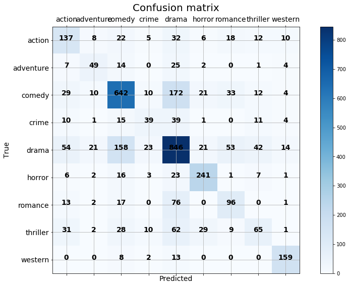
Confusion Matrix
The confusion matrix can help us see where our model is going wrong by plotting predicted class values vs actual class values. It looks like ‘Drama’ and ‘Comedy’ are getting confused for each other, ‘Thriller’, ‘Adventure’, and ‘Crime’ movies are hard to pin down, often being confused for ‘Drama’. Ultimately, there are at least as many correct predictions than false predictions for each row of the matrix, so I’m happy with these results. Especially when considering that genre classification is a tricky task for many humans as well.
from sklearn.metrics import confusion_matrix

def plot_confusion_matrix(true,predicted,classes):
    import itertools
    cm=confusion_matrix(true,predicted,labels=classes)

    fig = plt.figure(figsize=(15,9))
    ax = fig.add_subplot(111)
    cax = ax.matshow(cm,cmap=plt.cm.Blues)
    plt.title('Confusion matrix',fontdict={'size':20})
    fig.colorbar(cax)

    ax.set_xticklabels([''] + classes,fontdict={'size':14})
    ax.set_yticklabels([''] + classes,fontdict={'size':14})

    plt.xlabel('Predicted',fontdict={'size':14})
    plt.ylabel('True',fontdict={'size':14})

    plt.grid(b=None)
    fmt = 'd'

    for i, j in itertools.product(range(cm.shape[0]), range(cm.shape[1])):
        plt.text(j, i, format(cm[i, j], fmt),
             horizontalalignment="center",
             fontdict={'size':14,'weight':'heavy'})
classes = list(report.columns)[:-3]
plot_confusion_matrix(y_test,y_pred,classes)
Further Considerations
How can we make this model better? We can re-examine our tokenizing and lemmatizing. We only really did the bear minimum on that step. We could continue tuning the parameters of the model with grid-search.
Most importantly, we could choose a different metric to tune or model after taking into consideration what this model could be useful for. Maybe we want to use this model to recommend movies to users. If we know a user likes comedy, we might want to optimize for recall so that we can be sure that every comedy is represented in the output even if a few non-comedies make it through. If a user only likes drama and hates comdedy, we could optimize for precision to be sure that no comedies make it through. I chose weighted-F1 because it’s a balanced metric between precision and recall, and the results show that. But if we really want to apply this to the real world, we’ll need to think further about what really matters to end-users and other stakeholders.